
MAM5-INUM - Commande optimale
TP 1 - Navigation problem (a.k.a. Zermelo-Markov-Dubins)
Special thanks: P. Negre & M. Sadak (Polytech Nice Sophia)
One considers a ship in a constant current, \(0 \leq w \lt 1\). The angle of the velocity (wrt. to the water) is controlled, leading to the following dynamics:
\[ \begin{array}{rcl} \dot{x}(t) &=& w+\cos\theta(t),\quad t \in [0,t_f]\\ \dot{y}(t) &=& \sin\theta(t),\\ \dot{\theta}(t) &=& u(t). \end{array} \]
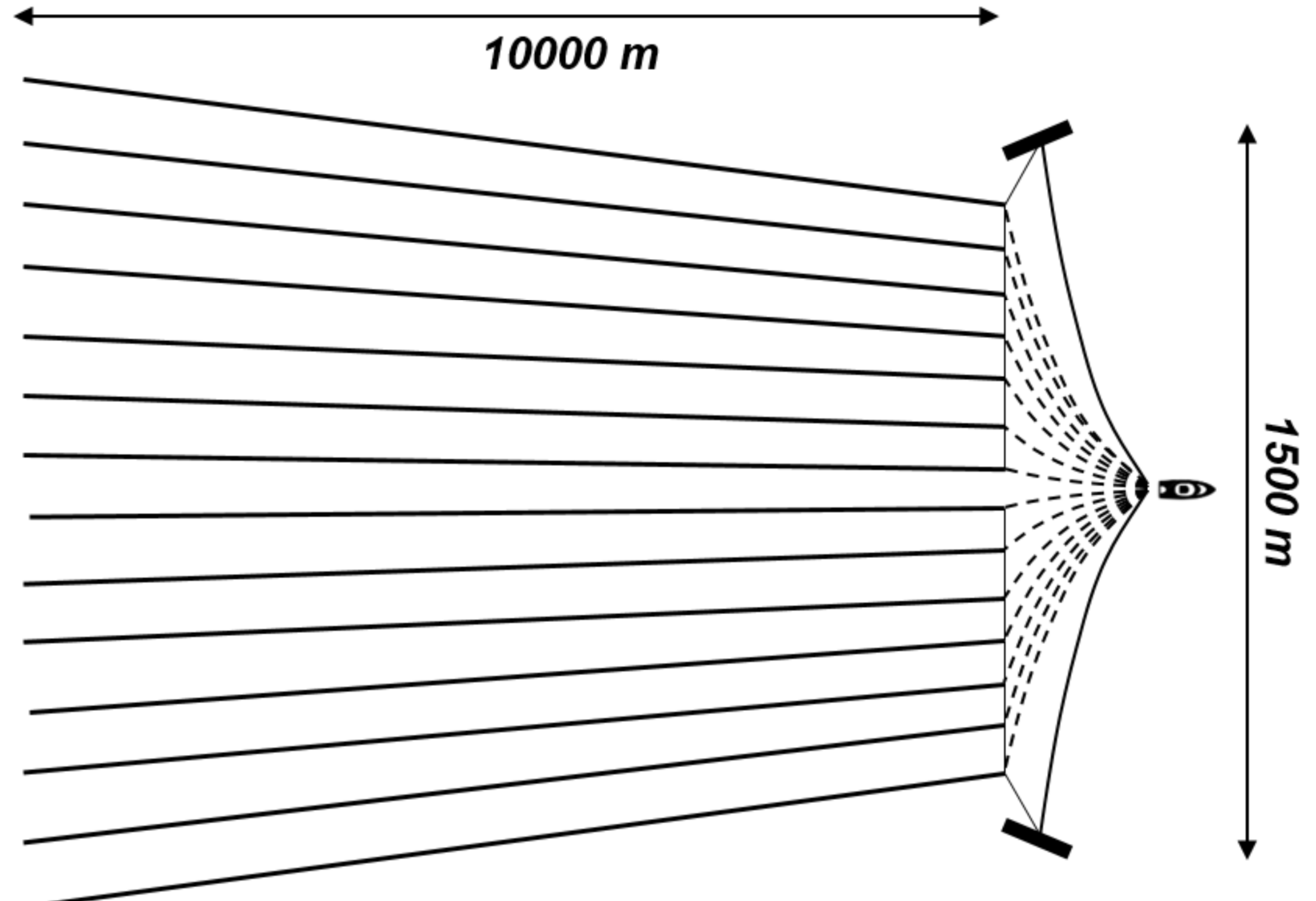
The turning rate (= curvature of turns) is limited, so \(|u(t)| \leq 1\). There boundary conditions at \(t=0\) and \(t=t_f\) on the position \((x,y)\) and on the angle \(\theta\) of the velocity in the water referential. The final time is to be minimised. The problem originates from a collaboration with the French company CGG that is interested in optimal maneuvers for very large ships doing marine prospection.
#JuMP model, Ipopt solver
using JuMP, Ipopt, Plots

sys = Model(optimizer_with_attributes(Ipopt.Optimizer,"print_level"=> 5))
set_optimizer_attribute(sys, "tol", 1e-8)
set_optimizer_attribute(sys, "max_iter", 500)

# Parameters
w = 0.5
x0 = 0
y0 = 0
θ0 = π/7
xf = 5
yf = 7
θf =-π/2
P = 100
Δt = 1/P

# Bounds for variables

@variables(sys,begin
    x[1:3, 1:P]           # x
    y[1:3, 1:P]           # y
    θ[1:3, 1:P]           # theta
    -1 ≤ u[1:3] ≤ 1       # u1 to u3, piecewise constant control
     0 ≤ τ[1:3]           # tau1 to tau3, length of subintervals
    end)

# Objective
@objective(sys, Min, τ[1]+τ[2]+τ[3])

# Constraints
@constraints(sys, begin
    x[1, 1] == x0
    y[1, 1] == y0
    θ[1, 1] == θ0
    x[2, 1] == x[1, P]
    y[2, 1] == y[1, P]
    θ[2, 1] == θ[1, P]
    x[3, 1] == x[2, P]
    y[3, 1] == y[2, P]
    θ[3, 1] == θ[2, P]
    x[3, P] == xf
    y[3, P] == yf
    θ[3, P] == θf
    end)

# Dynamics: Crank-Nicolson scheme
for j in 1 : P-1
    @NLconstraints(sys, begin
        # x' = w + cos(theta)
        x[1, j+1] == x[1, j] + 0.5 * τ[1]*Δt * ( w + cos(θ[1, j]) + w + cos(θ[1, j+1]) )
        x[2, j+1] == x[2, j] + 0.5 * τ[2]*Δt * ( w + cos(θ[2, j]) + w + cos(θ[2, j+1]) )
        x[3, j+1] == x[3, j] + 0.5 * τ[3]*Δt * ( w + cos(θ[3, j]) + w + cos(θ[3, j+1]) )
        # y' = sin(theta)
        y[1, j+1] == y[1, j] + 0.5 * τ[1]*Δt * ( sin(θ[1, j]) + sin(θ[1, j+1]) )
        y[2, j+1] == y[2, j] + 0.5 * τ[2]*Δt * ( sin(θ[2, j]) + sin(θ[2, j+1]) )
        y[3, j+1] == y[3, j] + 0.5 * τ[3]*Δt * ( sin(θ[3, j]) + sin(θ[3, j+1]) )
        # theta' = u
        θ[1, j+1] == θ[1, j] +       τ[1]*Δt * u[1]
        θ[2, j+1] == θ[2, j] +       τ[2]*Δt * u[2]
        θ[3, j+1] == θ[3, j] +       τ[3]*Δt * u[3]
    end)
end

# Solves for the control and state
println("Solving...")
status = optimize!(sys)
println("Solver status: ", termination_status(sys))
x1 = value.(x)'[:]
y1 = value.(y)'[:]
θ1 = value.(θ)'[:]
u1 = [ value.(u)[1]*ones(P); value.(u)[2]*ones(P); value.(u)[3]*ones(P) ]
τ1 = value.(τ)
println("Cost: " , objective_value(sys))
println("tf: ", τ1[1]+τ1[2]+τ1[3], "\t τ: ", τ1)

# Plots: states and control
t = zeros(3*P)
t[1:P] = τ1[1]*(0:P-1)
t[P+1:2*P] = P*τ1[1] .+ τ1[2]*(0:P-1)
t[2*P+1:3*P] = P*(τ1[1]+τ1[2]) .+ τ1[3]*(0:P-1)
t = Δt * t
x_plot = plot(t, x1, xlabel = "t", ylabel = "position x", legend = false, fmt = :png)
y_plot = plot(t, y1, xlabel = "t", ylabel = "position y", legend = false, fmt = :png)
θ_plot = plot(t, θ1, xlabel = "t", ylabel = "θ", legend = false, fmt = :png)
u_plot = plot(t, u1, xlabel = "t", ylabel = "control", legend = false, fmt = :png)
display(plot(x_plot, y_plot, θ_plot, u_plot, layout = (2,2)))

# Plots: trajectory with heading arrows
step = 5
idx = 1:step:length(x1)
L = 2.0 # constant arrow length (data units)
ux, uy = L * cos.(θ1[idx]), L * sin.(θ1[idx])

traj_plot = plot(x1, y1; c=:black, lw=3, aspect_ratio=:equal, size=(600,600), legend=false)
scatter!(traj_plot, x1[idx], y1[idx]; c=:red)
quiver!(traj_plot, x1[idx], y1[idx]; quiver=(ux, uy), c=:blue)
display(traj_plot)

# Animation: progression along the curve
xl = extrema(x1) .+ (-1, 1)
yl = extrema(y1) .+ (-1, 1)
anim = @animate for k in eachindex(idx)
    plot(x1, y1; c=:lightgray, lw=3, aspect_ratio=:equal, size=(600,600), legend=false, xlims=xl, ylims=yl)
    plot!(x1[1:idx[k]], y1[1:idx[k]]; c=:black, lw=3)
    scatter!(x1[idx[1:k]], y1[idx[1:k]]; c=:red)
    quiver!(x1[idx[1:k]], y1[idx[1:k]]; quiver=(ux[1:k], uy[1:k]), c=:blue)
end
gif(anim, "trajectory.gif", fps=10)